NanoDreamer: Learning to Act Through Imagination
Recently, I've been getting into world models and embodied intelligence, and because I love video games, obviously Dreamer caught my attention. However, I had one problem. I have no GPU.
So what do I do instead? Build my own tiny Dreamer, small enough to train on my MacBook. And because I wanted to understand every piece, I started from the bottom with my own autograd engine, tensor library, neural network layers, optimizers, and transformer.
After a lot of debugging, that became NanoDreamer! A 750k-parameter world model and actor–critic that learns to play all 5 MinAtar games, with the actor trained entirely through imagination and a model small enough to run and train on my M5! It trains from scratch on its own gameplay, without expert demonstrations or game-specific strategies, using the same architecture and training setup with separate weights for each game.
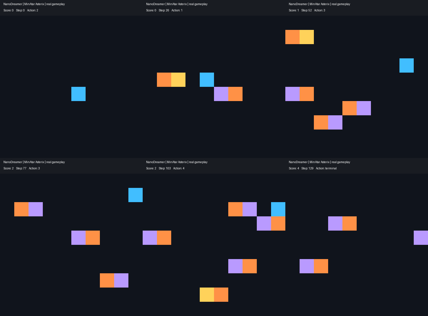
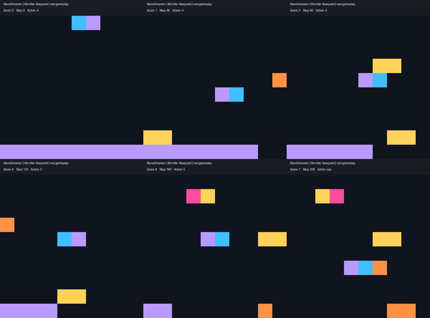
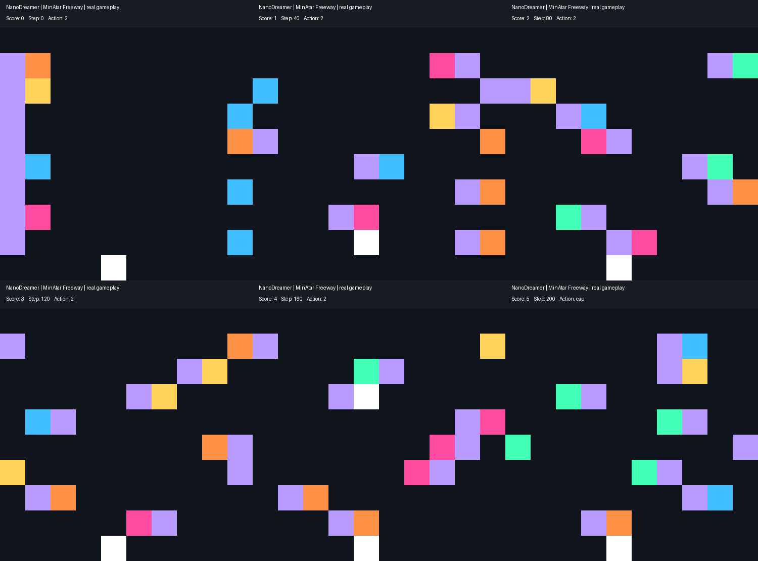
Here's NanoDreamer playing all 5 games after 500k steps per game (around 3 hours on an M5 Pro).
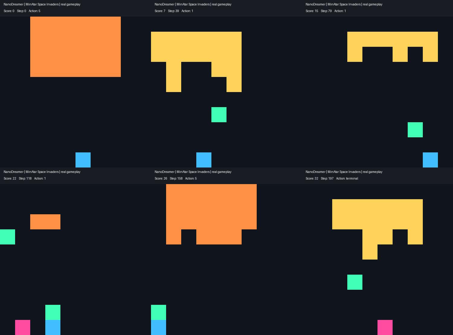
Move your cannon along the bottom, shoot the descending aliens, and dodge their shots. A hit from an alien or enemy shot ends the game.
- Your cannonalong the bottom row
- Alienscolor indicates their movement direction
- Your shotstravel upward
- Enemy shotstravel downward
+1 for each alien shot. Moving, firing, and surviving a step do not give extra points.
In this write-up I'll show you the bugs, experiments, and architectural changes it took to get Dreamer working at a fraction of the cost. If you're new to ML, I also wrote a separate guide to the foundations, with my own implementation and learnings!
How hard could it be?
I started by reading DreamerV3 and DreamerV4, trying to figure out what I actually needed to build. The idea seemed simple enough. A world model learns how the game works, an actor chooses actions inside its predictions, and a critic estimates the rewards beyond them. Here's what my first attempt looked like.
I started with an MLP autoencoder that compressed each frame into a 64-dimensional latent embedding. Once it could reconstruct the screen, I froze its weights.
A small causal transformer read the latent embeddings alongside action and positional embeddings. Its three prediction heads estimated the next latent state, reward, and probability the game would continue. The actor and critic were MLPs that saw the current latent concatenated with its change from the previous frame.
The actor then trained through 5-step imagined rollouts, sampling an action and feeding each predicted latent back into the model. We combined the predicted rewards with the critic's estimate of future return to give the actor feedback on its actions.
In my head, this all worked in theory. Now I just had to see whether it actually would.
Inside the first draftArchitecture, losses, and imagined returns
First, describe the game in 64 numbers
A small MLP autoencoder compressed each game frame into 64 numbers, then tried to reconstruct it.
Most cells were empty. A model could therefore get many cells right by predicting an almost empty screen. I used weighted binary cross-entropy to make missing an occupied cell more costly.
Open any equation to see what the symbols mean.
I then froze the autoencoder. The transformer had to work with whatever those 64 numbers preserved.
Then, predict what an action does
The transformer read eight steps of latent and action history. It had two causal blocks, with width 64 and four attention heads.
Three heads read the output. The next-latent head predicted a change to the current latent. The reward head predicted a number, and the continuation head predicted the probability that the episode kept going.
The predicted-frame loss decoded the predicted latent and compared it with the real next frame. Cells that changed received more weight, so a small moving object was harder to ignore. I combined the four losses like this.
Now, let the actor practise
I started with real history from replay. The actor chose an action, the frozen model predicted the next latent, reward, and continuation, and the actor chose again. I repeated this for five imagined actions.
The critic estimated rewards beyond the five-step window. Assuming the episode continues, a simple return adds predicted rewards to that final estimate.
The actual script used lambda returns, mixing the next critic estimate with the longer return. I used γ = 0.99 and λ = 0.95. Here s is the actor–critic input state.
Each decision got its own return target. I subtracted what the critic had expected to get the advantage. A positive advantage made the sampled action more likely, while a negative one made it less likely.
These are the core losses. An entropy bonus encouraged exploration. The targets were detached, and actor gradients flowed through action probabilities, not through the world model.
But fitting imagined returns does not make them right. I later checked the critic against discounted returns from real gameplay.
Uh, it did not work
The first training run used roughly 20,000 steps. And it didn't even shoot.. a complete disaster. Across 30 games, it averaged only 0.03 points. Even a random policy scored 4.3.
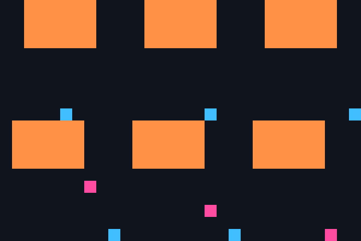
My first doubt was whether the model was predicting the rewards the actor needed to learn from. I replayed the same actions in the real game and the model, then compared what actually happened with what it predicted.
Here is an example I took from the experiment.
The model was quite off with its reward predictions. The model expected about 1.19 points on step four, but the actual shot earned one point on step five, when the model predicted almost nothing. It even predicted small negative rewards when nothing was earned. The actor was being given the wrong answer to learn from. D:
Across more trajectories, reward timing quickly deteriorated beyond one step into the future.
One step ahead, about 72% of the reward events were timed correctly. Eight steps ahead, that was only about 1%. The model could start from a real history, but its imagined future quickly became unreliable.
Those unreliable imagined rewards could also distort the critic's predictions. In one diagnostic, its average estimate was 10.46, while real discounted returns averaged only 3.16. So the actor could be learning from both misplaced rewards and an overly optimistic critic.
Changing how the model learned
The model could start from a real history, but struggled once it had to continue from its own predictions. I had two ideas for improving that experience: learn from the actor's actual gameplay and train on several predicted steps.
First, the model had only seen random gameplay, so it might struggle in situations our actor reached. I added the actor's real gameplay to replay so the model could learn from those mistakes.
repeat with the new policy ↻
Second, our earlier probe showed predictions falling apart further into the future. I tested whether training on several predicted steps, rather than one step from a real history, would help.
The idea was simple: feed each predicted latent back into the model to predict the next step, then compare the predictions against the real latents using the recorded actions. In this experiment, I fine-tuned the model for 600 updates on five-step rollouts.
In the separate five-step check, 600 rollout updates reduced latent prediction error by about 18% and reward prediction error by about 9%. Not bad! But better predictions didn't necessarily mean a better agent.
I combined online replay and rollout training and tried Space Invaders again. The run reached around 4 points in roughly 50k steps and... plateaued from there.
Better than 0.03, but still close to random. I needed to check whether the model was really what held it back.
Taking a little inspiration
The initial training changes hadn't been enough. I went back to older DreamerV2 concepts and used them alongside the diagnostics to rethink how the model represented the game and learned from experience.
Read the screen with shared filters. A projectile could appear in any column, so I replaced the MLP with a CNN. Instead of learning each position separately, it could reuse the same filters across the screen.
Practise the futures it would learn from. Our earlier diagnostics showed predictions drifting during imagination. I kept three-step generated rollouts so the predictor practised using its own outputs. I also sampled rare reward events more often, with importance weights correcting the sampling bias.
Well, did it fix it?
The architecture looked more complete, but did it actually predict rewards better? I replayed identical actions through the early and rebuilt Space Invaders models to check. Using trajectories from 30 random-play games, both started with eight real frames and predicted eight steps.
Across 1,314 rollout windows, here is how often each model put a real reward event on the right step.
- Better timing. Five steps ahead, correctly timed events increased from 6 of 95 to 40 of 95.
- Closer reward totals. Five-step cumulative reward error fell from 0.313 to 0.125, about 60% lower.
- Still some imaginary points. False alarms at step five increased from 6 to 27. The rebuilt model found more real rewards, but also predicted more that never happened.
A big success! Now, you'd expect the imagined frames to look better too, right? Here is the same shot through both models, with the real game on top and each model's decoded predictions below. Hover over a heatmap to see its decoded frame.
Interestingly enough, the first draft actually matched these particular frames more closely, even though the rebuilt model predicted rewards better across the larger test. A cleaner-looking imagined screen wasn't the same as a more useful reward prediction.
If you're interested, I also did a deeper dive into the model-training choices and their effects.
The final draft
Better predictions were only useful if the actor could learn from them. The rebuild also changed how the actor and critic used the model. These were already part of the checkpoint tested above; here's how they fit together.
- Shared history. The actor and critic had only seen the current latent and a one-frame change. I gave them the transformer's summary of up to 16 frames and preceding actions, so both could use a longer history to choose actions and estimate future rewards.
- An action MLP. Previously, the action went into the transformer. Now this MLP combines the history summary with the chosen action before predicting the next latent, reward, and continuation. The actor can choose from the history before the model predicts that action's consequences.
- Real targets for the critic. I added real replay returns alongside imagined ones to help ground its optimistic estimates. It still guides the actor through return targets, shown by the dashed training path.
Inside the working versionArchitecture, losses, and imagined returns
First, describe the game in 64 numbers
The CNN encoder compresses each frame into 64 numbers. Shared 3 × 3 filters look for local patterns across the grid. The decoder reconstructs the observation channels using weighted binary cross-entropy.
Unlike the first draft, prediction losses also update the encoder. A slowly moving target encoder provides the real latent targets, so the predictor isn't chasing every encoder update immediately.
Open any equation to see what the symbols mean.
Reconstruction checks what the latent preserves visually. Prediction losses give it feedback about the consequences the world model needs to learn.
Then, predict what an action does
The transformer reads up to 16 frames and preceding actions. It has two causal blocks, width 128 and four attention heads. A small MLP combines its summary hₜ with the current action before the three prediction heads.
The heads predict the next latent, a reward distribution over 255 bins, and continuation probability. Each generated step checks all three, plus the frame decoded from the predicted latent.
Three generated steps feed predictions back into the model. A quarter of sampling draws come from reward events, with importance weights correcting that mixture. Padding is excluded from losses.
Now, let the actor practise
The actor and critic read the transformer's history summary. Starting from replay, the actor chooses five imagined actions. The model predicts their rewards and continuation probabilities, and the target critic estimates what comes afterward.
Actions with returns above the critic's expectation become more likely. A running return scale keeps the advantage comparable as rewards change, and a small entropy bonus encourages exploration.
This recipe trains the critic on three-step real replay returns, bootstrapped with a target critic, plus a smaller imagined-return loss. The actor still learns entirely in imagination.
After 4,000 initial random transitions, the actor keeps collecting real gameplay. Every eight policy steps, I update the world model, actor, and critic. Exploration falls from 40% random actions to a 5% floor, so the agent can still try something outside its current preference and learn from the result.
The moment we've been waiting for
The predictions were better. Now for the test that mattered—could an actor learning inside them play the real game? Here are the training runs for Space Invaders and Breakout.
Space Invaders
Breakout
Finally, something was working. At 200k steps, Space Invaders scored nearly 3× random and Breakout nearly 7× random. But would the same recipe work across the rest of MinAtar?
With the algorithm working, I trained it for 500,000 policy steps on each MinAtar game, using separate weights but the same architecture and hyperparameters. Here are the resulting scores, averaged over 100 fresh games per agent.
Average game score · higher is better
And there it was. The same roughly 750k-parameter architecture, trained separately on each MinAtar game, beat the random baseline across the board. After the failed runs, misplaced rewards, and nights spent debugging, NanoDreamer was finally learning to play through imagination. :D

Takeaways and next steps
NanoDreamer changed what I pay attention to when reading a paper. I started by looking at architecture diagrams. Now I'm much more interested in the assumptions, training data, and experiments behind the results.
It also taught me to be more careful about what an experiment actually tells me. Getting an agent to work and understanding why it works are different achievements. I'm happy we reached the first, but there's still work to do on the second.
For my next project, I want to spend less time recreating a complete system and more time investigating a specific question. What information does a latent representation lose? When does an imagined rollout become unreliable, and can the agent recognize that?
But I'm also tempted to just build more working algorithms and architectures through my favourite video games, like Smash Ultimate or Deadlock. We'll see where that takes me!
And lastly, thank you for reading! I really appreciate you making it this far. I spent way too many sleepless nights debugging this thing and pulled an all-nighter to finish the write-up, so it means a lot if you enjoyed it!
Additional notes
Extra experiments, hyperparameters, and my training and evaluation setup.
Game rewards
I used the rewards supplied by MinAtar, without custom shaping. There are no extra points for firing, moving, or surviving a step.
| Game | What earns reward | What ends the game |
|---|---|---|
| Space Invaders | +1 for each alien shot. | An alien reaches or hits the cannon, or an enemy shot hits it. |
| Breakout | +1 for each brick broken. | The paddle misses the ball. |
| Asterix | +1 for each treasure collected. | The player touches an enemy. |
| Seaquest | +1 for each enemy shot. Surfacing with six divers adds a bonus based on remaining oxygen. | An enemy or bullet hits the submarine, oxygen runs out, or it surfaces without a diver. |
| Freeway | +1 for reaching the top of the road. | The environment timer expires. A car hit resets the chicken to the bottom; it doesn’t end the episode. |
Scores are sums of these rewards. The games have different scoring opportunities, so a score of 5 means something different in each game. Sampling reward events more often changes the training data mix; reward bins change how the model predicts a number. Neither adds rewards to the environment.
Our rollout limits can also end a recorded episode before the environment itself ends. Freeway’s own timer is longer than our 1,000-action final evaluation limit.
Working-version hyperparameters
These are the settings for the full rebuilt recipe behind the five-game results. Each game uses the same settings and architecture, with separate weights trained from scratch.
| Setting | Value |
|---|---|
| Latent size | 64 |
| CNN channels | 16 → 32 → 64, with 3 × 3 filters |
| Transformer | Width 128 · 2 blocks · 4 attention heads |
| History context | 16 steps |
| Reward / value distributions | 255 bins, symlog range −5 to 5 |
| World-model / real-return horizon | 3 steps |
| Actor imagination horizon | 5 steps |
| World-model batch | 32 replay contexts |
| Imagination batch | 64 starting contexts |
| Initial random experience | 4,000 environment actions |
| Update frequency | 1 world, actor, and critic update per 8 policy steps |
| Replay capacity | 200,000 transitions |
| Reward-event sampling mixture | 25% event starts + 75% uniform starts, importance-corrected |
| Optimizer | Adam |
| World-model learning rate | 0.0002 |
| Actor learning rate | 0.00004 |
| Critic learning rate | 0.0001 |
| Gradient norm clipping | 5 for each optimizer |
| Discount γ / return mixing λ | 0.99 / 0.95 |
| Actor entropy coefficient | 0.001 |
| Policy probability mixing | 99% learned probabilities + 1% uniform |
| Random-action exploration | 40% initially, falling to a 5% floor by 26,250 policy steps |
| Target encoder / critic update | 1% / 2% toward the current network per update |
| Generated-step loss weights | Latent 1 · frame 1 · reward 2 · continuation 0.2 |
| Critic loss weights | Real replay 1 · imagined 0.3 |
The controlled comparisons change the named encoder, critic, or sampling choice. Their settings should not be confused with the full recipe above.
Training and evaluation details
A policy step means one action taken in the real environment. The 500k-step runs contain 500,000 policy actions, plus 4,000 initial random actions. Imagined transitions and gradient updates do not count toward that number. Each training episode allows up to 1,000 actions.
| Result | Evaluation |
|---|---|
| Longer-run learning curves | 100 games per checkpoint · 200-action limit · different evaluation seeds at each checkpoint |
| Final five-game table | 500k training steps · 100 fresh games per game · 1,000-action limit |
| Training-choice comparison charts | Matched 150k training steps · 100 games · evaluation seed 920000 · 200-action limit |
| Training-choice endpoint checks | 300 games · evaluation seed 940000 · 200-action limit; one run ended at 184,712 training steps |
The agent samples its learned action probabilities during evaluation, without the additional training-time random-action exploration. Random baselines use the same game, evaluation seeds, and action limits as the corresponding agent check.
The five-game results have one training seed per game. The additional comparisons include two seeds for some recipes and one for others. More evaluation games reduce uncertainty about a saved policy; they don’t establish reliability across training seeds. The 32-point clip is a selected episode, not the average.
Additional training comparisons
After the longer runs, I went back to check which training signals helped the policy. I compared versions with one signal removed, then followed up on the promising alternatives. The actor learned entirely in imagination throughout.
All comparisons below use 150k real policy steps and the same 100 evaluation games, with a 200-action limit. That keeps the training budget equal, including the run that later hit its time cap.
Did prediction errors need to train the encoder?
My original encoder learned to reconstruct frames. Reconstructing a projectile didn't necessarily make its next collision easy to predict, so the full rebuild also let prediction losses train the encoder.
To test that choice, I trained another version where the CNN learned only reconstruction. The architecture stayed the same, and the encoder still learned online. It just stopped receiving gradients from the prediction losses.
| Game | Joint encoder | Reconstruction only |
|---|---|---|
| Space Invaders | 9.32 | 11.26 |
| Breakout | 2.92 | 2.98 |
In this first seed, reconstruction-only training scored higher in Space Invaders and almost the same in Breakout. So I couldn't credit joint encoder training for the improvement. A representation learned through reconstruction was still competitive in this setup.
Did the critic benefit from real rewards?
Remember the critic expecting more reward than the real game gave? In the full rebuild, I tried grounding it with real replay returns alongside imagined targets. That sounded useful, but the actor was practising inside the model. I wanted to check whether the mixed targets actually helped.
I compared that critic with one trained entirely on imagined returns, then repeated both versions with a fresh training seed. Each dot below is a separately trained agent.
Space Invaders
Breakout
In Space Invaders, imagination-only critic training improved the score in both seeds. In Breakout, it helped in the first seed but not the second. Giving the critic real targets wasn't a consistently better choice.
What if I combined the simpler choices?
That left a follow-up worth trying. What happened if the encoder learned only reconstruction and the critic learned only in imagination? I tested that combination in the second seed.
| Game | Full recipe | Imagined critic | + Reconstruction encoder |
|---|---|---|---|
| Space Invaders | 11.16 | 15.14 | 12.59 |
| Breakout | 1.48 | 1.40 | 5.08 |
In Breakout, the combination reached 5.08, while the other two versions stayed around 1.4–1.5. In Space Invaders, it beat the full version but stayed behind the imagination-only critic with a jointly trained encoder.
So the changes weren't simply additive. I had promising simpler alternatives, but no single recipe had established itself as the most reliable across games. The combined version had only one seed; these comparisons measured the effects of the training choices, not the mechanism behind them.
The architecture detours
I tried more capacity because the predictor might not have been able to track objects and delayed rewards. Increasing transformer width from 64 to 128 and blocks from 2 to 3 grew the world model from roughly 109,000 to 613,000 parameters. Some reward metrics improved, but gameplay didn't improve consistently.
I also tried a small RSSM for recurrent memory. Spatial-token experiments kept four regions separate instead of compressing a frame into one token, and a separate denoising experiment refined a noisy next-state guess over several steps. Those were attempts to preserve local detail and model more complicated futures, inspired by DreamerV4.
These trials didn't isolate which architecture was best. They used different checkpoints and training conditions, and some runs were short. The detailed log preserves them, but they don't establish a single architectural cause for the early failures.
Inside the small RSSM trial
RSSM stands for recurrent state-space model. Our trial used a 64-number recurrent memory and 8 groups of 8 categorical choices. A GRU-like transition updated the memory from the previous stochastic state and action. A prior predicted the next stochastic state from memory, while a posterior could also use the real observation to correct that prediction.
The decoder, reward head, and continuation head read the combined memory and stochastic state. Training used image reconstruction, reward and continuation losses, and balanced KL losses to bring the prior and posterior together. In imagination there was no new observation, so only the prior was available. This was a compact DreamerV3-inspired trial, not the original DreamerV3 model size.
There was also a replay bug in one RSSM trial. Replay required eight-step windows and discarded shorter episodes, including the actor's six-step failures. In one random dataset, 231 of 300 episodes were too short. The rebuilt replay keeps short terminal windows and masks padding, so those failures remain training examples.
After 2,000 updates on 1,000 random episodes, the Space Invaders prior missed all 73 one-step reward windows in the held-out probe, even though the observation-conditioned loss had improved. That was a failure of this implementation and training setup, not evidence that small RSSMs cannot work.
References
- MinAtar — the environments used to train and evaluate the agents.
- DreamerV2 — Mastering Atari with Discrete World Models
- DreamerV3 — Mastering Diverse Domains through World Models
- DreamerV4 — Training Agents Inside of Scalable World Models
- Raj Ghugare’s PyTorch DreamerV2 implementation — a reference for the CNN encoder and replay setup.
Want to build it from scratch?
Follow the foundations, from algebra and gradients to the networks behind the agent.
Read the foundations →